E1n1verse

Photo Published & Cashing Cheques

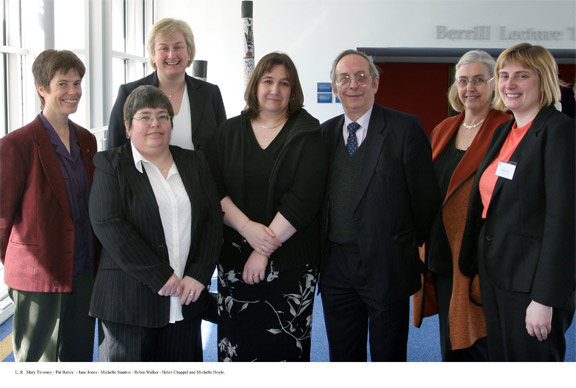
Here's a picture of me (and 6 others) who were recently honoured with the first teaching awards ever available for associate lecturers at the Open University in the United Kingdom. In the picture, I'm wearing a black suit and a salmon-coloured top on the far right of the picture. A version of this picture just appeared in an article the May-June edition of Open House, the OU-wide newspaper for staff of the Open University.

In previous years, the awards were only open to support staff and full-time central academic staff which is reflected in the headline for the article of "AL's honoured at last." Alas, while I am mentioned by name in the article, they don't say very much about any of us. For example, about me. all they said is "Winnings [sic] ALs pictured are ... TT280 and TT281 tutor Michelle Hoyle." Yep, that's it. We all had a few words in the article.

The cheque arrived in the most recent pay advice and I'm busy plotting what "personal" and "professional" self-development use I can put it to. I've started with a new pedometer and a new scale (waiting for the bank transfer to clear and that to be shipped still), and am trying to justify one of those new AirPort Express portable wireless stations with support for streaming to my stereo. I was also considering retroactively including the cost of my rather expensive Rosetta Stone language learning software for German; that's definitely personal development.

Oh, the agony of deciding!

Metric MDS & Data Delivered

I had a good meeting with Thufir on May 14th, lasting almost the full allotted hour. This was because I've recently had a breakthrough with my MATLAB analysis and can quantitatively evaluate the similarity between different people or different algorithms with my multi-dimensional scaling (MDS) diagrams. I took some output to the meeting which compared my half-baked algorithm against the cosine normalization version. Both use hypernyms, but how they weigh the hypernyms is different. My automated analysis algorithm also produces an MDS cluster diagram as output for each of the data files provided (see anal1ahyper and anal2ahyper).

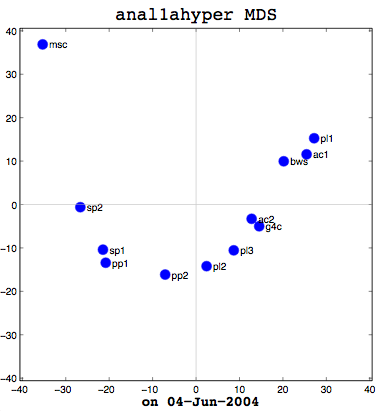
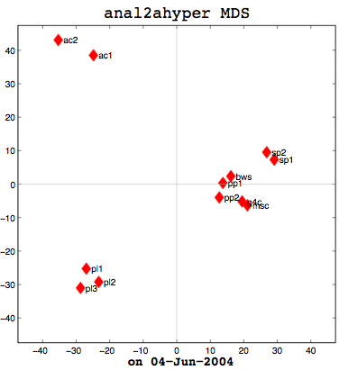
Anal1a, in terms of clumping, doesn't look very good, at least not anymore. That was not previously the case, but I had revised my algorithm to make it symmetrical as per the insructions of a computing statistician here at the University of Sussex. He claimed that the Procrustes Rotation needed symmetric data and my nonsymmetric data, where Doc1 vs Doc2 didn't have the same similarity as Doc2 vs Doc1, was not going to work. That change has, I believe, altered the efficacy of the algorithm and things are no longer clumped together as promisingly as they were previously. The clumps should be a two- or three-letter short code followed by a digit. Therefore, ac1 and ac2 belong together. Pl1, pl2, and pl3 belong together, and so on. The clumping is significantly better in the already symmetric cosine normalization algorithm (anal2a). The two speech processing documents are clumped together (sp1 and sp2), all of the Power PC and G4 documents are together (pp1, pp2, g4c), and the three Pine Lake tornado stories are clumped far away from everything else (which is all computer-related) and together on their own. Excellent clumping, in fact. So the hypernym hypothesis looks like, on these short documents, it is working well with cosine normalization.

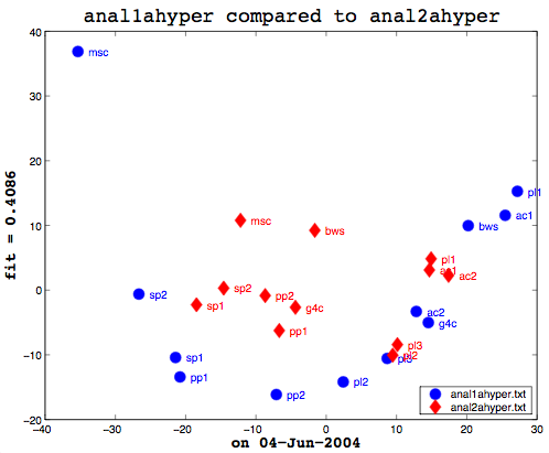
Here's the final bit of loveliness: comparing one MDS cluster diagram against another. MDS output is mapped to the vector space independently. That is, the same data will produce the same visualization or mapping, but different data is mapped to a different vector space, so you cannot just compare one MDS matrix to another directly. That is where Procrustes Rotation comes in. It applies a series of intelligent matrix transformations, trying to map the second vector matrix onto the source vector matrix. As a side benefit, essential in my case, it always provides a fitness measure to tell you how close the two were. on a scale of 0 to 1. So these two, as you can see (see above image), even after the transformations, were not that close together. As it happens, though, this is not particularly useful information to know. I am currently more interested in assessing how close the two algorithms are to human classifiers.

This recent success gave us plenty to discuss, particularly with respect to metric and non-metric data. The MDS community calls source data metric when the similarity or dissimilarity data is symmetric. That is, the value at row 2, column 1 is the same as the value at row 1, column 2. Classical multi-dimensional scaling (MDS) is designed to only work with metric data. SPSS includes the ALSCAL and PROXSCAL MDS algorithms which can work with non-metric data, but MATLAB's classical MDS does not because it treats things as Eucledean distances--another reason why I had to alter the Anal1a algorithm. The primary reason I now had metric data for everything, however, was because the computing statistician had told me I needed it for the Procrustes. Hawever, as we were examining my output, it occurred to me that Procrustes did not really care if the data was symmetric, so long as the dimensions of the data were the same (the same number of rows and columns). Which leads us to question whether the application of the method is statistically sensible or not. To that end, I need to track down a new computing statistician and perhaps a mathematician and discuss the process with them. My original computing statistician has retired.

Earlier I said that comparing one machine to another, to see how they fit is not useful information, but what would be interesting is to prepare a matrix of all the possible combinations of human judgements, cosine normalization, and weird formula:

                      cosine   wrd form.   human
cosine (anal2a)		x
weird formula (anal1a)           x
human                                        x

So that is my task for my next meeting (on the 16th of June). Before then, I need to figure out how to get MATLAB to take multiple tables as data. In SPSS, I could paste in several tables (representing all of the people's individual data, for example) and it would work with that. That is necessary in order to aggregate the peopel to do the comparison. Onward ho, then! Progress at last!

Dirty Data Done Dirt Cheap

I have to confess to feeling a bit stupid. I have been struggling with MATLAB for weeks now, trying to get it to read in my data files so I can automate my analyses. My data is in a tab-delimited file and looks something like:

	Doc1	Doc2	Doc3	Doc4
Doc1	100	76	18	91
Doc2	76	100	22	35
Doc3	18	22	100	65
Doc4	91	34	65	100

This is not too dissimilar from the labelled diagram, part of the MATLAB documentation on data importing. Except that, if you look at the table below it, which describes which functions to use, they don't have a function with a similar example to their labelled diagram. Early on I thought I should be able to use dlmread, which allows you specify rows/columns for starting points or a range. My idea was just to have a range which excluded the non-numeric troublesome labels. No matter what I did, though, I could not get it to work. It was frustrating, because I could paste the data into the Import Wizard and that could handle the data fine. I wrote people, I researched on the web, and I tried all sorts of things.

Eventually, I came full-circle back to dlmread and experimented by making a small data file with unrelated data in it. That worked fine. So I then copied half of one of my data tables into the test file and tried that. That also worked fine. I copied the whole data table into the test file and used dlmread on it. It worked fine! What was the difference between the two identical data files other than their filenames? When I uncovered the answer to that, I kicked myself. My data files were generated years ago and stored on my Mac OS 9-based laptop. My laptop and the data have since migrated to Apple's swoopy BSD-based UNIX goodness and that's the environment that MATLAB runs under. So... Have you guessed the problem? Yes, it was linefeeds! The data files had original Mac linefeeds and MATLAB wanted UNIX linefeeds. D'oh! It just goes to reaffirm that the things you don't see can really hurt you.

Once that was solved, work proceded rapidly apace as I was now able to finish automating the whole comparison process from start to finish.

function  [Anal1Raw, Anal2Raw, Anal1MDS, Anal2MDS, fit] = 
      processEinCiteData(firstFile, secondFile, runName, labels)


% Read in the similarity matrices from the two data files
Anal1Raw = dlmread(firstFile, '\t', 1, 1);
Anal2Raw = dlmread(secondFile, '\t', 1, 1);

% Set up default document name labels if we didn't get any
if nargin < 4
	labels = {'g4c', 'pp1', 'pp2', 'msc', 'pl1', 'pl2', 'pl3', 'sp1', 'sp2', 'ac1', 'ac2', 'bws'};
    if nargin < 3
    runName = '';
    end
end

% Set up labels for the filenames
fileName1 = regexprep(firstFile, '\..*$', '');
fileName2 = regexprep(secondFile, '\..*$', '');

% Convert the similarity data to numbers below 1 for use in MDS
Anal1Raw = abs(100 - Anal1Raw) 
Anal2Raw = abs(100 - Anal2Raw) 

% Calculate the MDS and prepare a diagram showing the
% clusterings for the first document
[Anal1MDS, eigvals] = cmdscale(Anal1Raw);
figure(1);
plot(1:length(eigvals),eigvals,'bo-');
graph2d.constantline(0,'LineStyle',':','Color',[.7 .7 .7]);
axis([1,length(eigvals),min(eigvals),max(eigvals)*1.1]);
xlabel('Eigenvalue number');
ylabel('Eigenvalue');
plot(Anal1MDS(:,1),Anal1MDS(:,2),'bo', 'MarkerFaceColor', 'b', 'MarkerSize', 10);
axis(max(max(abs(Anal1MDS))) * [-1.1,1.1,-1.1,1.1]); axis('square');
text(Anal1MDS(:,1)+1.5,Anal1MDS(:,2),labels,'HorizontalAlignment','left');
hx = graph2d.constantline(0,'LineStyle','-','Color',[.7 .7 .7]);
hx = changedependvar(hx,'x');
hy = graph2d.constantline(0,'LineStyle','-','Color',[.7 .7 .7]);
hy = changedependvar(hy,'y');
title(['\fontname{lucida}\fontsize{18}' fileName1 ' MDS']);
xlabel(['\fontname{lucida}\fontsize{14}' runName ' on ' date], 'FontWeight', 'bold');

% Calculate the MDS and prepare a diagram showing the
% clusterings for the second document
[Anal2MDS, eigvals] = cmdscale(Anal2Raw);
figure(2);
plot(1:length(eigvals),eigvals,'rd-');
graph2d.constantline(0,'LineStyle',':','Color',[.7 .7 .7]);
axis([1,length(eigvals),min(eigvals),max(eigvals)*1.1]);
xlabel('Eigenvalue number');
ylabel('Eigenvalue');
plot(Anal2MDS(:,1),Anal2MDS(:,2),'rd', 'MarkerFaceColor', 'r', 'MarkerSize', 10);
axis(max(max(abs(Anal2MDS))) * [-1.1,1.1,-1.1,1.1]); axis('square');
text(Anal2MDS(:,1)+1.5,Anal2MDS(:,2),labels,'HorizontalAlignment','left');
hx = graph2d.constantline(0,'LineStyle','-','Color',[.7 .7 .7]);
hx = changedependvar(hx,'x');
hy = graph2d.constantline(0,'LineStyle','-','Color',[.7 .7 .7]);
hy = changedependvar(hy,'y');
title(['\fontname{lucida}\fontsize{18}' fileName2 ' MDS']);
xlabel(['\fontname{lucida}\fontsize{14}' runName ' on ' date], 'FontWeight', 'bold');

% Apply Procrustes to the two MDS results to map them 
% into the same vector space and prepare a plot of the 
% result
[fit, Z, transform] = procrustes(Anal1MDS, Anal2MDS);
figure(3);
plot(Anal1MDS(:,1), Anal1MDS(:,2), 'bo','MarkerFaceColor', 'b', 'MarkerSize', 10);
hold on
plot(Z(:,1), Z(:,2), 'rd', 'MarkerFaceColor', 'r', 'MarkerSize', 10);
hold off
text(Anal1MDS(:,1)+1.5,Anal1MDS(:,2), labels, 'Color', 'b');
text(Z(:,1)+1.5,Z(:,2),labels, 'Color', 'r');
xlabel(['\fontname{lucida}\fontsize{14}' runName ' on ' date], 'FontWeight', 'bold');
ylabel(['\fontname{lucida}\fontsize{14}' 'fit = ' num2str(fit, '%2.4f')], 'FontWeight', 'bold');
titleStr = ['\fontname{lucida}\fontsize{18}' fileName1 ...
        ' compared to ' fileName2];
title(titleStr, 'HorizontalAlignment', 'center', ...
    'VerticalAlignment', 'bottom');
legend({firstFile, secondFile}, 4);

At the end, I had a quantitative number, the degree of fit, between two diagrams after applying the Procrustes Rotation to them. Finally! On a whim, I fed in the same data table as both arguments to my comparison program. That is, I compared the same data file to itself. My hypothesis was that the resultant degree of fit should be either 0 or 1 (depending on which the fitness was measured). Much to my surprise, no matter which data file I used, the result was never 0 or 1. My previous Procrustes Analysis code was taken from some sample code in the MATLAB documentation and looked like: [D,Z] = procrustes(Anal1aMDS, Anal2aMDS(:,1:2)); That last bit in () is some kind of MATLAB scaling, which, being a novice to MATLAB, I didn't realize. So, in fact, my two diagrams weren't the same which is why I wasn't getting a 100% degree of fit. I do not want to say how long it took me to narrow that down. Once I did, though, it looked like I was basically set and I was able to quickly produce some comparisons between my "weird" half-baked metric and the cosine normalization one. One small step for EinKind.

This is a delayed entry from May 12th, 2004.

Conceptual Change

David Jonassen visited the IDEAs lab on May 11th from the University of Missouri to present a talk on "Model-Building for Conceptual Change (Cognitive Tools in Action)". While this isn't (or so I thought) related to my own research or interests in any way, we were all encouraged to attend if possible and I'm always interested in talks about learning in general. Here, belatedly, is a synopsis of my understanding of his presentation.

The key underlying principle seemed to emphasize having people fail in their problem solving attempt at some issue because then conceptual change has a change to be engaged and then students will learn. This failure need not be catastrophic; in fact, it probably should not be, I would say, or the failure would foster a strong sense of discouragement, which is not going to get a student into the "learning zone." So, how do you put students into a non-threatening environment where they can safely experiment and fail? David Jonassen's idea was to encourage them to engage in model building which demonstrates their conceptual understanding of the problem/issue at hand. When learners build models,their understanding of the problem domain is deepened because you cannot model what you do not understand. Model building also allows you, as the instructor, to view the learner's level of conceptual change as their models evolve. It is therefore possible to assess their underlying understanding without resorting to formal assessment tests. Finally, David Jonassen suggested that model building also improves critical reasoning and thinking because model building forces the model builder to examine the process and problem solving methodology.

David Jonassen researches (among other things) the use of technology in educational settings to improve understanding. More information on his approaches to problem solving are available from on the following web site page: http://tiger.coe.missouri.edu/~jonassen/PB.htm.

I think this is some interesting research, but obviously not applicable to every learning situation. Physical processes, like volcanos, weather, chemical reactions, etc. are very appropriate for model building. Or maybe I just need to change my understanding of what constitutes a model? For example, I'm teaching students how to program in JavaScript. In a way, a program is sort of like a model and we give students programming projects where they model some kind of answer to a stated problem to demonstrate their understanding of the process. Most students do not implement the solution correctly intially, so they need to refine their understanding of the problem and its solution over several iterations. Failure is forcing them into a state of conceptual change and as they repair their assumptions and their "model" code, they are learning valuable lessons about what works and the process of both developing and fixing. I guess, in fact, I've been doing this all along; I just didn't have a name for it!