E1n1verse

WoW Survey Deisgn: Putting the Horse Before the Cart?

I've been thinking about the design of the study I want to do on motivation in World of Warcraft. My immediate approach, similar to introductory programming students, was to jump right into the meat of it and start writing survey questions instead of planning. In order to get the data you need in the study, you need to know what questions you want answered. You need to plan. Without knowing that, how can you write survey questions to elicit those answers? So what is it I want to know?

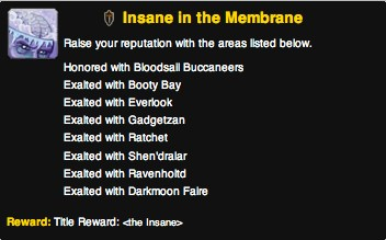
I want to say something about the kinds of motivations people have for playing World of Warcraft. Specifically, I want to enumerate factors that motivate players to persist in the game even when it involves tasks that are repetitive, boring, or seemingly impossibly long. For example, there's an achievement in World of Warcraft called "Insane in the Membrane" that gives the completer a reward of an in-game title of "The Insane." This achievement requires you to raise your reputation points with different game factions to exalted, the highest level. Generally, you need about 21,000 points to reach exalted. Points are gained by completing quests, collecting and turning in items, or sometimes killing certain types of things. If you only had to gain exalted reputation with one or two factions, this would not be difficult. However, you need to do this with eight different factions, most of which are not factions you would be accruing large amounts of reputation with during the normal course of play. To increase the difficulty, several of the factions involved have rival factions. With those factions, as you gain reputation with one, you lose reputation points with the rival faction, making the process of completing this achievement complex in addition to time-consuming. The WoWWiki (2009) page describes some strategies for completing this achievement and the complexities of the faction-rival relationships.

Most tasks players undertake are not going to be as complex, time-consuming, or mind-numbing to complete as the aptly-named "Insane in the Membrane". There are, however, many smaller day-to-day activities necessary for successful raiding or to get some particular piece of gear, such as doing daily quests to earn gold, or harvesting materials for potions or enchantments, or completing instance and after instance to get badge rewards or reputation rewards. I'm making it sound like getting achievements or gear is the be-all, end-all, but I think the situation is more complex than that. It's that hypothesis I want to verify.

Other things I would like to be able to comment on include the relationships between gender and motivation, or motivation and age, or possibly even motivation and nationality. I do not necessarily believe there will be a relationship between motivation and nationality necessarily, but how can you definitively say if you do not look for the correlation? That gives me the following questions I want answered:

1. What motivates people to play World of Warcraft?
2. What motivates people to persist in very boring or difficult tasks?
3. Is there a relationship between gender and stated motivations? If so, what is it?
4. Is there a relationship between age and stated motivations? If so, what is it?
5. Is there a relationship between nationality and stated motivations? If so, what is it?
6. Is there a relationship between character roles and classes and motivation?

With those six questions in mind and the original study idea of determining motivation via analysis of free-form essays about motivation, I can now go ahead and develop the specific survey questions that will help elicit data to answer those questions. Going back to considering my approach-whether I should start with planning versus start with survey question-it was not as clearcut as I expected. By starting with some potential survey questions and then thinking about the answers I would get from them, I gained a better idea about what answers I wanted, a kind of iterative development process. Sometimes putting the horse first helps you know where and how to put the cart!

References:

WoWWiki. (2009) Insane in the Membrane, [online] WoWWiki. Available from http://www.wowwiki.com/Insane_in_The_Membrane (Accessed November 6, 2009).

Metric MDS & Data Delivered

I had a good meeting with Thufir on May 14th, lasting almost the full allotted hour. This was because I've recently had a breakthrough with my MATLAB analysis and can quantitatively evaluate the similarity between different people or different algorithms with my multi-dimensional scaling (MDS) diagrams. I took some output to the meeting which compared my half-baked algorithm against the cosine normalization version. Both use hypernyms, but how they weigh the hypernyms is different. My automated analysis algorithm also produces an MDS cluster diagram as output for each of the data files provided (see anal1ahyper and anal2ahyper).

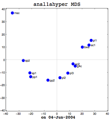
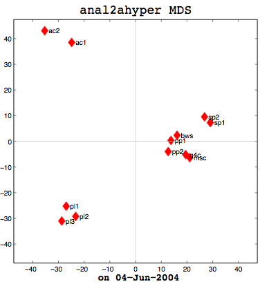
Anal1a, in terms of clumping, doesn't look very good, at least not anymore. That was not previously the case, but I had revised my algorithm to make it symmetrical as per the insructions of a computing statistician here at the University of Sussex. He claimed that the Procrustes Rotation needed symmetric data and my nonsymmetric data, where Doc1 vs Doc2 didn't have the same similarity as Doc2 vs Doc1, was not going to work. That change has, I believe, altered the efficacy of the algorithm and things are no longer clumped together as promisingly as they were previously. The clumps should be a two- or three-letter short code followed by a digit. Therefore, ac1 and ac2 belong together. Pl1, pl2, and pl3 belong together, and so on. The clumping is significantly better in the already symmetric cosine normalization algorithm (anal2a). The two speech processing documents are clumped together (sp1 and sp2), all of the Power PC and G4 documents are together (pp1, pp2, g4c), and the three Pine Lake tornado stories are clumped far away from everything else (which is all computer-related) and together on their own. Excellent clumping, in fact. So the hypernym hypothesis looks like, on these short documents, it is working well with cosine normalization.

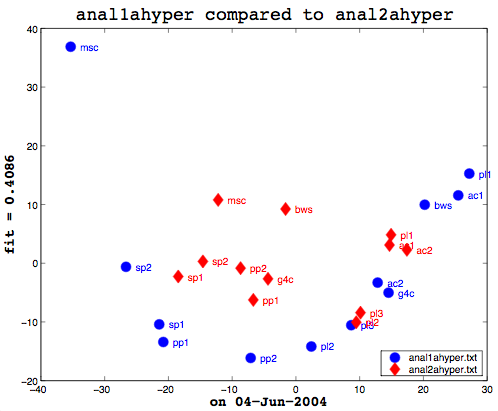
Here's the final bit of loveliness: comparing one MDS cluster diagram against another. MDS output is mapped to the vector space independently. That is, the same data will produce the same visualization or mapping, but different data is mapped to a different vector space, so you cannot just compare one MDS matrix to another directly. That is where Procrustes Rotation comes in. It applies a series of intelligent matrix transformations, trying to map the second vector matrix onto the source vector matrix. As a side benefit, essential in my case, it always provides a fitness measure to tell you how close the two were. on a scale of 0 to 1. So these two, as you can see (see above image), even after the transformations, were not that close together. As it happens, though, this is not particularly useful information to know. I am currently more interested in assessing how close the two algorithms are to human classifiers.

This recent success gave us plenty to discuss, particularly with respect to metric and non-metric data. The MDS community calls source data metric when the similarity or dissimilarity data is symmetric. That is, the value at row 2, column 1 is the same as the value at row 1, column 2. Classical multi-dimensional scaling (MDS) is designed to only work with metric data. SPSS includes the ALSCAL and PROXSCAL MDS algorithms which can work with non-metric data, but MATLAB's classical MDS does not because it treats things as Eucledean distances--another reason why I had to alter the Anal1a algorithm. The primary reason I now had metric data for everything, however, was because the computing statistician had told me I needed it for the Procrustes. Hawever, as we were examining my output, it occurred to me that Procrustes did not really care if the data was symmetric, so long as the dimensions of the data were the same (the same number of rows and columns). Which leads us to question whether the application of the method is statistically sensible or not. To that end, I need to track down a new computing statistician and perhaps a mathematician and discuss the process with them. My original computing statistician has retired.

Earlier I said that comparing one machine to another, to see how they fit is not useful information, but what would be interesting is to prepare a matrix of all the possible combinations of human judgements, cosine normalization, and weird formula:

                      cosine   wrd form.   human
cosine (anal2a)		x
weird formula (anal1a)           x
human                                        x

So that is my task for my next meeting (on the 16th of June). Before then, I need to figure out how to get MATLAB to take multiple tables as data. In SPSS, I could paste in several tables (representing all of the people's individual data, for example) and it would work with that. That is necessary in order to aggregate the peopel to do the comparison. Onward ho, then! Progress at last!

Dirty Data Done Dirt Cheap

I have to confess to feeling a bit stupid. I have been struggling with MATLAB for weeks now, trying to get it to read in my data files so I can automate my analyses. My data is in a tab-delimited file and looks something like:

	Doc1	Doc2	Doc3	Doc4
Doc1	100	76	18	91
Doc2	76	100	22	35
Doc3	18	22	100	65
Doc4	91	34	65	100

This is not too dissimilar from the labelled diagram, part of the MATLAB documentation on data importing. Except that, if you look at the table below it, which describes which functions to use, they don't have a function with a similar example to their labelled diagram. Early on I thought I should be able to use dlmread, which allows you specify rows/columns for starting points or a range. My idea was just to have a range which excluded the non-numeric troublesome labels. No matter what I did, though, I could not get it to work. It was frustrating, because I could paste the data into the Import Wizard and that could handle the data fine. I wrote people, I researched on the web, and I tried all sorts of things.

Eventually, I came full-circle back to dlmread and experimented by making a small data file with unrelated data in it. That worked fine. So I then copied half of one of my data tables into the test file and tried that. That also worked fine. I copied the whole data table into the test file and used dlmread on it. It worked fine! What was the difference between the two identical data files other than their filenames? When I uncovered the answer to that, I kicked myself. My data files were generated years ago and stored on my Mac OS 9-based laptop. My laptop and the data have since migrated to Apple's swoopy BSD-based UNIX goodness and that's the environment that MATLAB runs under. So... Have you guessed the problem? Yes, it was linefeeds! The data files had original Mac linefeeds and MATLAB wanted UNIX linefeeds. D'oh! It just goes to reaffirm that the things you don't see can really hurt you.

Once that was solved, work proceded rapidly apace as I was now able to finish automating the whole comparison process from start to finish.

function  [Anal1Raw, Anal2Raw, Anal1MDS, Anal2MDS, fit] = 
      processEinCiteData(firstFile, secondFile, runName, labels)


% Read in the similarity matrices from the two data files
Anal1Raw = dlmread(firstFile, '\t', 1, 1);
Anal2Raw = dlmread(secondFile, '\t', 1, 1);

% Set up default document name labels if we didn't get any
if nargin < 4
	labels = {'g4c', 'pp1', 'pp2', 'msc', 'pl1', 'pl2', 'pl3', 'sp1', 'sp2', 'ac1', 'ac2', 'bws'};
    if nargin < 3
    runName = '';
    end
end

% Set up labels for the filenames
fileName1 = regexprep(firstFile, '\..*$', '');
fileName2 = regexprep(secondFile, '\..*$', '');

% Convert the similarity data to numbers below 1 for use in MDS
Anal1Raw = abs(100 - Anal1Raw) 
Anal2Raw = abs(100 - Anal2Raw) 

% Calculate the MDS and prepare a diagram showing the
% clusterings for the first document
[Anal1MDS, eigvals] = cmdscale(Anal1Raw);
figure(1);
plot(1:length(eigvals),eigvals,'bo-');
graph2d.constantline(0,'LineStyle',':','Color',[.7 .7 .7]);
axis([1,length(eigvals),min(eigvals),max(eigvals)*1.1]);
xlabel('Eigenvalue number');
ylabel('Eigenvalue');
plot(Anal1MDS(:,1),Anal1MDS(:,2),'bo', 'MarkerFaceColor', 'b', 'MarkerSize', 10);
axis(max(max(abs(Anal1MDS))) * [-1.1,1.1,-1.1,1.1]); axis('square');
text(Anal1MDS(:,1)+1.5,Anal1MDS(:,2),labels,'HorizontalAlignment','left');
hx = graph2d.constantline(0,'LineStyle','-','Color',[.7 .7 .7]);
hx = changedependvar(hx,'x');
hy = graph2d.constantline(0,'LineStyle','-','Color',[.7 .7 .7]);
hy = changedependvar(hy,'y');
title(['\fontname{lucida}\fontsize{18}' fileName1 ' MDS']);
xlabel(['\fontname{lucida}\fontsize{14}' runName ' on ' date], 'FontWeight', 'bold');

% Calculate the MDS and prepare a diagram showing the
% clusterings for the second document
[Anal2MDS, eigvals] = cmdscale(Anal2Raw);
figure(2);
plot(1:length(eigvals),eigvals,'rd-');
graph2d.constantline(0,'LineStyle',':','Color',[.7 .7 .7]);
axis([1,length(eigvals),min(eigvals),max(eigvals)*1.1]);
xlabel('Eigenvalue number');
ylabel('Eigenvalue');
plot(Anal2MDS(:,1),Anal2MDS(:,2),'rd', 'MarkerFaceColor', 'r', 'MarkerSize', 10);
axis(max(max(abs(Anal2MDS))) * [-1.1,1.1,-1.1,1.1]); axis('square');
text(Anal2MDS(:,1)+1.5,Anal2MDS(:,2),labels,'HorizontalAlignment','left');
hx = graph2d.constantline(0,'LineStyle','-','Color',[.7 .7 .7]);
hx = changedependvar(hx,'x');
hy = graph2d.constantline(0,'LineStyle','-','Color',[.7 .7 .7]);
hy = changedependvar(hy,'y');
title(['\fontname{lucida}\fontsize{18}' fileName2 ' MDS']);
xlabel(['\fontname{lucida}\fontsize{14}' runName ' on ' date], 'FontWeight', 'bold');

% Apply Procrustes to the two MDS results to map them 
% into the same vector space and prepare a plot of the 
% result
[fit, Z, transform] = procrustes(Anal1MDS, Anal2MDS);
figure(3);
plot(Anal1MDS(:,1), Anal1MDS(:,2), 'bo','MarkerFaceColor', 'b', 'MarkerSize', 10);
hold on
plot(Z(:,1), Z(:,2), 'rd', 'MarkerFaceColor', 'r', 'MarkerSize', 10);
hold off
text(Anal1MDS(:,1)+1.5,Anal1MDS(:,2), labels, 'Color', 'b');
text(Z(:,1)+1.5,Z(:,2),labels, 'Color', 'r');
xlabel(['\fontname{lucida}\fontsize{14}' runName ' on ' date], 'FontWeight', 'bold');
ylabel(['\fontname{lucida}\fontsize{14}' 'fit = ' num2str(fit, '%2.4f')], 'FontWeight', 'bold');
titleStr = ['\fontname{lucida}\fontsize{18}' fileName1 ...
        ' compared to ' fileName2];
title(titleStr, 'HorizontalAlignment', 'center', ...
    'VerticalAlignment', 'bottom');
legend({firstFile, secondFile}, 4);

At the end, I had a quantitative number, the degree of fit, between two diagrams after applying the Procrustes Rotation to them. Finally! On a whim, I fed in the same data table as both arguments to my comparison program. That is, I compared the same data file to itself. My hypothesis was that the resultant degree of fit should be either 0 or 1 (depending on which the fitness was measured). Much to my surprise, no matter which data file I used, the result was never 0 or 1. My previous Procrustes Analysis code was taken from some sample code in the MATLAB documentation and looked like: [D,Z] = procrustes(Anal1aMDS, Anal2aMDS(:,1:2)); That last bit in () is some kind of MATLAB scaling, which, being a novice to MATLAB, I didn't realize. So, in fact, my two diagrams weren't the same which is why I wasn't getting a 100% degree of fit. I do not want to say how long it took me to narrow that down. Once I did, though, it looked like I was basically set and I was able to quickly produce some comparisons between my "weird" half-baked metric and the cosine normalization one. One small step for EinKind.

This is a delayed entry from May 12th, 2004.

Love the License

By the end of April, I seemed to be stymied in my quest for an affordable copy of MATLAB that I could run on my local laptop. The university maintains a license pool for the base software plus toolkits. I do have access to run a copy from the license server when I'm on campus. It actually worked off of campus too, when I'd been told it shouldn't, but that turned out to be a mistake. When I reported it, the firewall was closed to the outside world for requests for the license server. That's where honesty gets you: no MATLAB accessibility from anywhere with an Internet connection.

I was hoping to snag one of the concurrent licenses for my permanent use and offered even to buy an additional one for that purpose as that would be cheaper. I was told that I couldn't have one and I should investigate the student version of the software. Unfortunately, the student version is only available to students in taught courses, not Ph.D. research students, so that wasn't any good. I mentioned to Thufir that I'd been turned down, reportedly by the head of software/hardware procurement within our department. Thufir promised to see what he could do. Then, last week, I received an e-mail last week from the lab manager, the person in charge of the procurement. He offered, if somebody would pay for it, to install an academic version of the software on my university-owned equipment for only £525 (~930 US/780 €). That was just for the base software and not also for the toolkit I need.

As I haven't met with Thufir since receiving the e-mail, I haven't discussed it with him to see if he's willing to cough up £525 (~930 US/780 €) plus £210 (~370 US/310 €) for the software for me. The lab manager stopped by my office today to see if somebody was going to pay for it and we entered into a discussion about the licensing arrangements. The academic license is only available for installation on university-owned equipment. I don't have any university-owned equipment. He doesn't want to be breaking the law by violating the terms of the licensing agreement which is fair enough. That does leave me in somewhat of a quandry: I don't qualify for the student edition; I'd be in violation of the license for an academic version; and I can't afford the £1625 (~2900 US/2400 €) commercial base software price plus an additional £600 (~1050 US/895 €) for the toolkit I need.

Why do I need my own copy? Can I live without my own copy? I can possibly do without my own copy as I can run it on campus, but I'm not on campus all the time. I do return to Canada for extended periods of time and we are investigating an option of moving back to Canada and having me commute out every quarter or so for a month as that would be cheaper than actually living here. Just last year I spent 6 months in Canada. Even if I am here, it's a problem if I just want to work from home. It would therefore be nice to have my own copy, but at what price?

I've told the lab manager that I'll get back to him. I'm meeting with Thufir on Friday. I also e-mailed MathWorks to ask about my situation and licensing arrangements for it. It does seem strange that their academic license is restricted by machine ownership rather than by reported use for the software. Their customer service auto-responder promises a response within 24 hours, but so far all I've received is the automatic response and a response from their database that my e-mail address has been updated in my profile. I have no idea what that's about. Maybe tomorrow will be better.

MATLAB & MDS

I need some help in using MATLAB and MDS, so I looked to Google to find resources. There seem to be more MDS resources than when I last looked quite some time ago. I found a useful page with links and pointers to MDS-related resources at http://www.granular.com/MDS/. From there, I obtained most of the resources for a pyschology course organized around MDS taught by one of the MDS's primary researchers Forrest Young. I downloaded all the notes in PDF format and stored them away to browse through. Young is the same researcher responsible for developing the ViSta software (Visual Statistics System), which looks a lot like that Canadian object-oriented, icon-based programming language. I remember looking at ViSta before, but I don't think it supported doing things like MDS and it hasn't been recently updated for anything other than Windows.

David L. Jones had a series of MATLAB pointers which included links to toolboxes for non-metric multidimensional scaling. The latter toolkit, developed by Mark Steyvers, doesn't come with any documentation and includes some DLLs, so I wonder if only works in Windows somehow? I couldn't find any other reference to it on the web.

I was waiting for the Mac support person to come install a new version of MATLAB for me. The demo installation and toolkits I installed last fall have long since expired. I'm also still waiting to hear back from the UNIX software support people in the department about acquiring one of the pool licenses for use with a copy of MatLab on my Macintosh off campus. Latish on in the day, I found the Mac support person and acquired a valid license file. It didn't work right off the bat. I had to edit the file and change the linefeeds from Macintosh ones to UNIX ones. After that, it worked great and it looks fantastic. So I should be able to start doing something with that soon. It also works from home, surprisingly enough, as long as I have an Internet connection, so that will be quite convenient. Hurrah! I am moving ahead.

Dimensional MATLAB Reading

Played around a little more with MATAB, although I didn't really get very far. I was trying to figure out how to use dlmread to import my data files properly into MATLAB automatically. It didn't really seem to want to fly somehow.

I spent some time trying to figure out how to automate my MATLAB work. I couldn't figure out how to get it to import the tab-delimited data files that my programs had produced using the dlmread command which should put it into a matrix. I can do it via the clipboard but not anyway else at the moment. Reviewing various MATLAB tutorials on the web, looking for hints, I realized that I need to review my understanding and knowledge of matrices again, so I've added this to my list of things to be done.

Assuming that my methodology is correct, which it might not be, I can now map one MDS cluttering onto another using the Procrustes in MATLAB. I need to figure out now how to get a single measure of how different the two are from that. I'm at least further along than before, so that's promising.

This is my current revised program:

% Import anal1ahyp.txt into anal1a matrix variable. Do this first! It's not done
% automatically here. Need first to do something like anal1a = abs(100 - anal1a) to
% get proper dissimilarity values to work with. The default ones in the files don't
% work as is.

docs = {'g4c', 'pp1', 'pp2', 'msc', 'pl1', 'pl2', 'pl3', 'sp1', 'sp2', 'ac1', 'ac2', 'bws'};
[Anal1aMDS, eigvals] = cmdscale(Anal1aRaw);
plot(1:length(eigvals),eigvals,'bo-');
graph2d.constantline(0,'LineStyle',':','Color',[.7 .7 .7]);
axis([1,length(eigvals),min(eigvals),max(eigvals)*1.1]);
xlabel('Eigenvalue number');
ylabel('Eigenvalue');
plot(Anal1aMDS(:,1),Anal1aMDS(:,2),'bx');
axis(max(max(abs(Anal1aMDS))) * [-1.1,1.1,-1.1,1.1]); axis('square');
text(Anal1aMDS(:,1),Anal1aMDS(:,2),docs,'HorizontalAlignment','left');
hx = graph2d.constantline(0,'LineStyle','-','Color',[.7 .7 .7]);
hx = changedependvar(hx,'x');
hy = graph2d.constantline(0,'LineStyle','-','Color',[.7 .7 .7]);
hy = changedependvar(hy,'y');

% Import anal2ahyp.txt into anal2a matrix variable. Do this first! It's not done
% automatically here.

Anal2aRaw = abs(100 - Anal2aRaw);
[Anal2aMDS, eigvals] = cmdscale(Anal2aRaw);

% do procustes
[D,Z] = procrustes(Anal1aMDS, Anal2aMDS(:,1:2));
plot(Anal1aMDS(:,1), Anal1aMDS(:,2), 'bo', Z(:,1), Z(:,2), 'rd');
text(Anal1aMDS(:,1)+0.5,Anal1aMDS(:,2), docs, 'Color', 'b');
text(Z(:,1)+0.5,Z(:,2),docs, 'Color', 'r');
xlabel('East of the Sun');
ylabel('West of the Moon');
legend({'Anal1a', 'Anal2a'}, 4);